OSITAI:

Optical Satellite Identification and Tracking System from Astronomical Images Using Feature Extraction and Machine Learning

Acess the paper (in Thai) ⎘

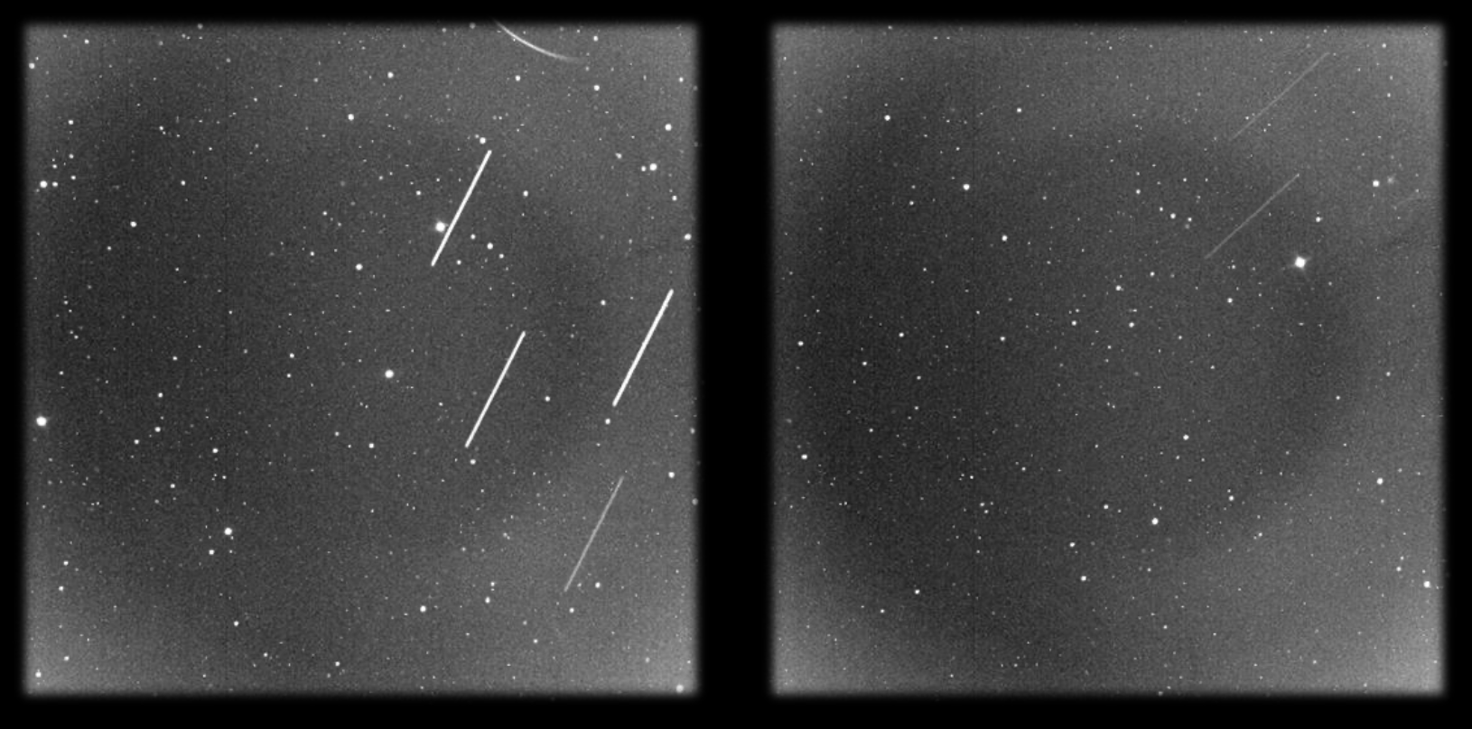
A satellite crosses a telescope’s field of view and leaves a streak across an astronomical image. Finding the streak is only the beginning. Identifying the object requires reconstructing the geometry of the image, the time of observation, the position of the telescope, and the satellite’s predicted orbit. An astronomical camera records light. A satellite identification system has to reconstruct the event that produced it.

This project, Optical Satellite Identification and Tracking System from Astronomical Images Using Feature Extraction and Machine Learning, explores how computer vision and orbital mechanics can work together to identify satellites in optical telescope observations.

Developed as a computer science senior project at Chulalongkorn University, the system combines image processing, U-Net segmentation, geometric feature extraction, astronomical coordinate transformations, and satellite orbital data. The objective is to move from pixels to a trajectory, and from a trajectory to a candidate identity. The distinction matters. A line detector can find a streak without knowing what produced it. An orbital model can predict where a satellite should appear without knowing whether the camera actually recorded it. Identification becomes possible only when the two agree.

1. The Problem: An Image Is Not an Identity

Objects orbiting Earth are observed for scientific, commercial, and security purposes. As the population of resident space objects grows, locating and identifying them becomes an increasingly important part of Space Situational Awareness (SSA). Optical telescopes offer one means of observing these objects. Unlike a system that depends on transmitting signals to a target, an optical observation records light reaching the telescope. During an exposure, a moving satellite can appear as a bright line against a background containing stars, galaxies, and noise.

The resulting image is both informative and ambiguous. A satellite trail may be faint, partially obscured, or discontinuous. Other image features can resemble sections of a trail. Even if a line is detected correctly, its shape alone does not establish which satellite produced it. A conventional workflow relies on knowing which objects are expected to pass through the observed region and comparing their predicted positions with the image. The difficulty is connecting a model of orbital motion with an imperfect photographic record.

There are three distinct problems.

First, the system must separate potential satellite trails from the astronomical background.

Second, it must reconstruct the geometry and direction of each detected trail.

Third, it must compare the observed trajectory with candidates calculated from orbital catalogues, accounting for the location and orientation of the telescope and the time of observation.

These problems cannot be solved independently. A correct line extracted from an image with incorrect pointing metadata can still lead to the wrong satellite identification. Detecting a streak is a computer vision problem. Identifying its source is a problem of geometry, time, and evidence.**

2. The Evidence: High-Resolution Astronomical Observations

The project uses astronomical video recordings captured with a ZWO ASI294MM Pro monochrome CMOS camera. The observations were collected on 15 February, 22 February, and 19 March 2026. The videos use RAW8 data and have a resolution of 8,288 × 5,644 pixels per frame. Depending on recording duration, the report describes video files ranging from approximately 5 to 20 GB.

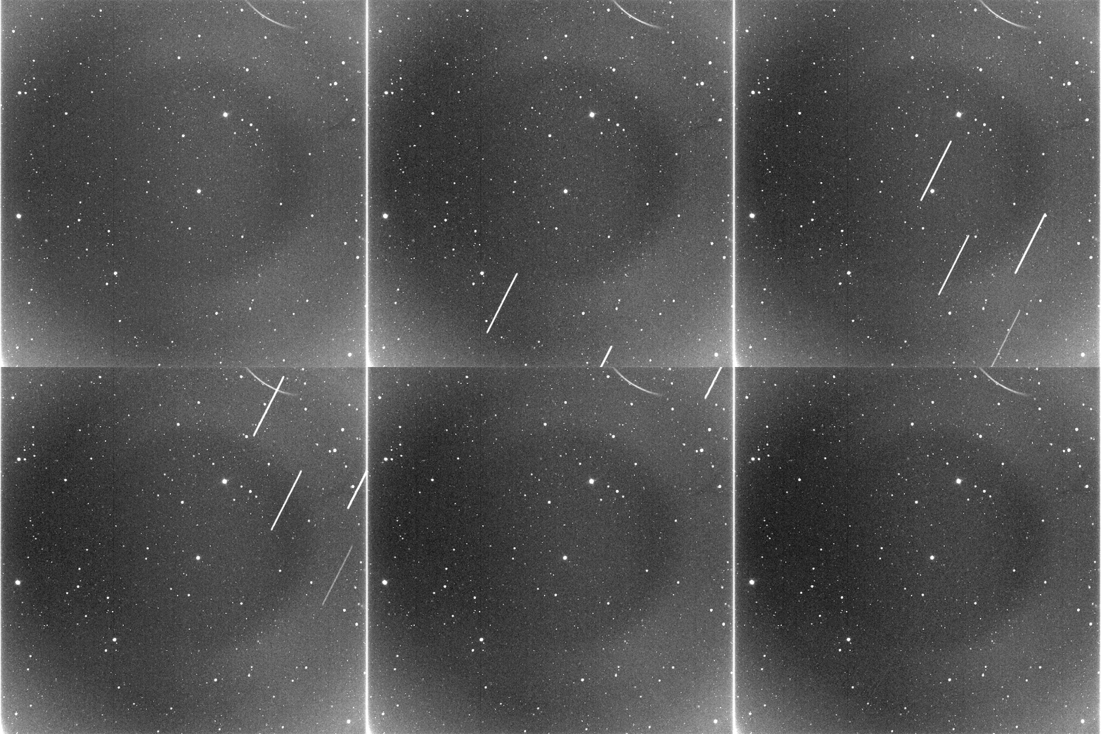
Each recording contains a sequence of observations rather than a single finished image. A satellite can occupy a different position in every frame, while stars generally appear as point-like sources. This temporal structure is useful. Combining information from multiple frames can reveal a longer and more continuous trail than any individual frame provides. It also creates a practical problem. Processing every pixel in every frame of a large video requires substantial computational and memory resources. The system therefore selects frames containing detectable trails for further analysis. The inputs consist of more than image data alone. The observation time, central pointing coordinates, field of view, telescope orientation, and observer location all contribute to the interpretation of a trail.

3. Extracting a Satellite Trail

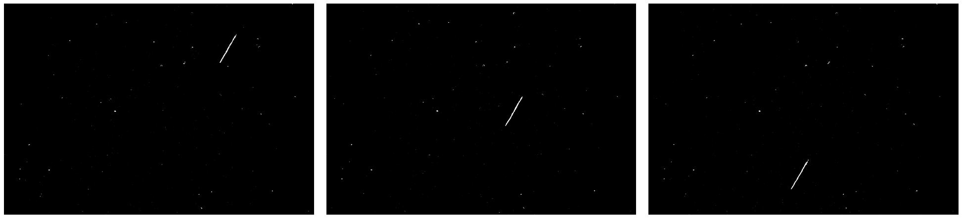
The image-processing pipeline begins by preparing the selected frames for segmentation. Each image is converted to grayscale and normalized so that variations in brightness can be handled more consistently. Images are padded where necessary to fit the patch dimensions expected by the segmentation model. The system then uses a U-Net model to identify pixels likely to belong to satellite trails. U-Net is an encoder-decoder neural network architecture commonly used for image segmentation. Rather than predicting a single label for an entire image, it produces a spatial prediction that distinguishes likely trail pixels from the surrounding background. The output is a probability map. Post-processing turns this map into a binary mask that can be used by subsequent geometric operations. The masks are cleaned using image-processing operations, including Gaussian smoothing, thresholding, morphological closing, and the removal of small connected components. These operations reduce isolated noise and help reconnect short gaps in a detected trail. The purpose is not to make the image visually attractive. It is to produce a representation of the trail that can be measured.

From individual frames to a continuous track

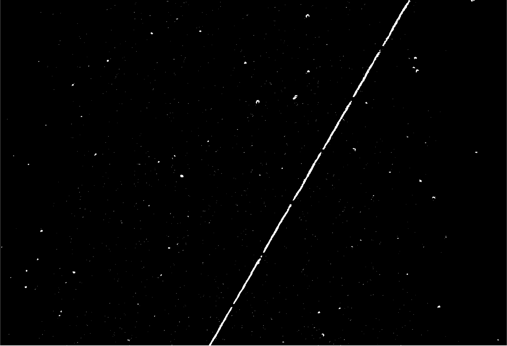
A satellite may not be equally visible throughout a recording. Atmospheric distortion, faint illumination, and background noise can interrupt the detected line. To address this, the system combines binary masks from multiple frames using a pixel-wise maximum operation. Where the satellite trail appears in successive frames, the merged mask accumulates evidence across those observations. The combined mask can then undergo further line extraction and refinement. Connected-component analysis helps isolate candidate structures. Line fitting estimates a dominant direction, while Hough-based line detection provides an alternative when the geometry is difficult to recover from the selected component.

The final representation includes the line’s endpoints, its equation, its length in pixels, and a motion vector describing its direction across the image. This converts a potentially fragmented visual feature into a geometric object that can be compared with a predicted trajectory.

4. The Camera Is a Coordinate System

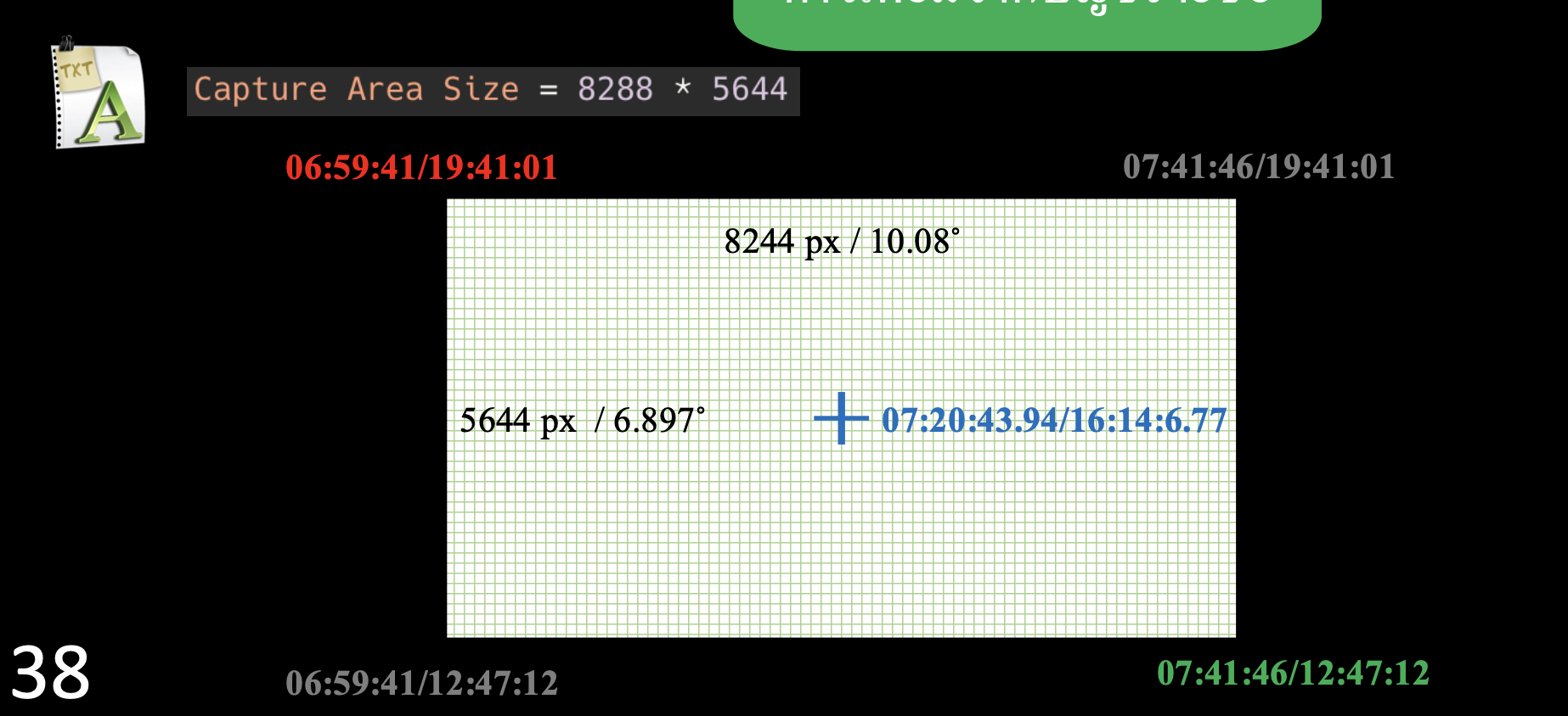
A line defined in image pixels has no immediate astronomical meaning. To compare it with an orbital prediction, the system must establish where the image lies on the celestial sphere. This is the transition from image geometry to astronomical coordinates. The project uses the image’s central right ascension (RA) and declination (Dec), its dimensions, and its field of view to construct a World Coordinate System (WCS). RA and Dec describe angular positions in the sky. Pixel coordinates describe positions within the camera sensor. WCS supplies the mathematical relationship between these representations. The implementation uses a tangent-plane projection, identified by the WCS coordinate types RA---TAN and DEC--TAN, together with the image centre and angular pixel scale.

The scale can be estimated from the angular width of the field of view divided by the image width. The central pixel becomes the reference point for the transformation, while the camera rotation determines the orientation of the image axes. The four image corners are then converted into sky coordinates to estimate the angular boundaries of the field of view. This establishes the region against which predicted satellite positions can be tested. The transformation depends on the accuracy of the input metadata. If the telescope was pointed somewhere other than the recorded coordinates, the WCS may describe a valid mathematical image of the wrong patch of sky. Coordinates are not incidental metadata. They are part of the measurement.

5. Reconstructing the Expected Orbit

The system needs an independent estimate of which satellites could have crossed the observed field of view. For this, the project uses Two-Line Element sets (TLEs) obtained from CelesTrak’s General Perturbations archive. The historical date is selected to correspond to the observation period, and the active-satellite catalogue is used as the candidate population.

TLEs encode orbital parameters in a standardized format. They are commonly used with the Simplified General Perturbations 4 (SGP4) model to calculate satellite positions at particular times. The project uses the Skyfield library to calculate those positions and transform them into coordinates relative to the observer. That calculation requires three pieces of information:

1. The satellite’s orbital data.
2. The observer’s geographical position and elevation, represented using WGS84.
3. The start and end times of the observation, expressed in Coordinated Universal Time (UTC).

Local Thai time is seven hours ahead of UTC, so timestamps must be converted consistently before the orbital calculations are performed. For each candidate satellite, the system calculates its apparent position at the beginning of the observation interval. Candidates outside the image’s angular boundaries are discarded. The positions of the remaining candidates are calculated again at the end of the interval to estimate their movement across the sky. The result is a predicted trajectory for each satellite that passes the initial spatial filter.

6. Matching Observed and Predicted Trajectories

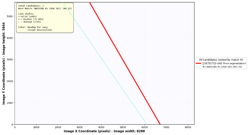
The experiments evaluated the system using six satellite observation datasets to assess its ability to combine image processing with orbital predictions for satellite identification. Overall, the results demonstrated that the system can detect satellite trails and identify corresponding objects when the observed trajectories align with predicted orbital paths. The most successful results were achieved when the trails were clear and the observation data were accurate and consistent.

The experiments also revealed that the system’s performance depends heavily on the quality of observation metadata and orbital information. Outdated orbital data can cause discrepancies between observed and predicted trajectories, while incorrect telescope coordinates can lead to misalignment. Similarly, unrecorded changes in telescope pointing can affect the consistency of multi-frame analysis, making it difficult to match detected trails with predicted satellite paths. Differences between observation timestamps and predicted passage times can also prevent correct identification, even when the object has been successfully detected.

Overall, the findings demonstrate that detecting an object does not necessarily guarantee its correct identification. Reliable satellite identification requires not only effective image processing but also accurate telescope coordinates, consistent pointing information, synchronized observation times, and up-to-date orbital data. These factors are essential for improving the system’s accuracy and reliability in practical applications.

8. A Model Cannot Repair Missing Evidence

The six test cases reveal a system whose results depend on the entire observation chain, not just the performance of its segmentation model.

The project successfully extracted line structures and calculated their equations and directions across the tested datasets. Two cases produced consistent initial identifications under the recorded observation conditions. In two additional cases, correcting the telescope’s central coordinates allowed the target to be identified. The remaining cases exposed unresolved difficulties involving changing pointing, candidate ambiguity, and timing.

These results should be understood within the limits of the experiment. Six datasets are not enough to establish general performance across every telescope, atmospheric condition, orbital regime, or observation workflow.

There are also several practical constraints. First, faint or noisy trails can remain incomplete after segmentation. The system may need more suitable observations or improvements in image acquisition to recover them reliably.

Second, the available computing resources limit the amount of footage that can be processed. Analysing more frames could improve the temporal continuity of a trail, although this also increases processing requirements.

Third, satellite identification depends on the quality and temporal relevance of TLE data. Historical orbital records can be incomplete, and using elements far from the observation date can introduce trajectory errors.

Fourth, telescope metadata must reflect the observation that actually occurred. Pointing changes, incorrect centre coordinates, inconsistent timestamps, and camera rotation can all distort the relationship between pixels and predicted sky positions.

These are not problems that can be solved by adding another layer to a neural network. Some require better instrumentation, more complete metadata, more historical orbital information, or a larger and more diverse observation dataset. The system is therefore best understood as a research prototype for optical satellite identification, rather than a fully operational space-surveillance platform.

9. Connect Measurements, Not Just Algorithms

The central idea behind this project is to connect computer vision with a physical model of the world. The image-processing stage identifies a possible trail. Geometric analysis reconstructs its direction and extent. WCS maps image coordinates to the sky. Orbital calculations estimate which satellites should have passed through that region. The final comparison evaluates whether the predicted and observed paths agree.

Each stage contributes evidence, and each stage has its own failure modes. A trail detector can be accurate while the camera metadata is wrong. An orbital model can be internally consistent while relying on outdated TLE data. A candidate can rank highly without the score representing a calibrated probability of identity. The system becomes useful when these components work together and when discrepancies are treated as information rather than concealed by a seemingly precise result. A line is an observation. An orbit is a prediction. Identification begins when the two can be reconciled.

Acess the paper (in Thai) ⎘

References

1. F. Stoppa et al. (2024). “Automated detection of satellite trails in ground-based observations using U-Net and Hough transform.” Astronomy & Astrophysics, 692, A199.

2. A. De Vittori, R. Cipollone, P. Di Lizia, and M. Massari (2022). “Real-time space object tracklet extraction from telescope survey images with machine learning.” Astrodynamics, 6(2), 205–218.

3. D. A. Vallado and P. J. Cefola (2012). “Two-line element sets – Practice and use.” 63rd International Astronautical Congress.

4. CelesTrak. General Perturbations data and historical satellite element sets. CelesTrak.

5. The Astropy Project. World Coordinate System and astronomical coordinate tools. Astropy.

6. Skyfield documentation. Satellite positions and astronomical calculations. Skyfield.